Analysis the data with Pivot Table in Google Sheet

Pivot table is the most commonly used function to do analysis data in sheets.

You can create a pivot table easily in google sheet with the data menu pivot commend.  Refer the picture.

 

 

The google sheet will create the pivot table in a new sheet; just select the required field in the right column of the pivot table.

Very simple steps with an added feature of sorting the value in pivot table in the options.

 

I have created a data sheet with a sample pivot table for you to understand it and work on the sheet to get practice of pivot table function.

 

In the sample data; I have also used a date and text function to fine the month representing the transactions.  You can use the function to create a meaning full pivot and reports can be generated easily.   Please give your feedback after using the sample data in the following data.

 

https://docs.google.com/spreadsheets/d/1dD8XmC8FKvxL2UTKM6maWuwaivyDmP-f5D4fFdfciYs/edit?usp=sharing

FREEZE TOP ROW TO VIEW HEADINGS OF A TABLE IN GOOGLE SHEET

GOOGLE SHEET - FUNCTIONS, It is easy to use and collaborate with our team.

At time we shall store the data in Google sheet.  When we scroll the data, the headings should be visible to us this function.

In the view menu, select the freeze button to get options of selecting the freeze the one row / multiple.  You can also freeze the column to scroll to the right.

I have given a sample data and menu example for ready reference.

Please follow the link:

https://docs.google.com/spreadsheets/d/1Uy_9LcsqKLYbmkUvi8Uq8M_BN9HHrlUvBluqT1OgWNA/edit?usp=sharing

Google Sheet - VLOOKUP Function

Google sheet is a good tool to work with our team and store our data safe.

How do we use the vlookup function in Google sheet.

vlookup function:

The function is used to pull the relevant/corresponding data from master table.

i.e. If you feed the role number of a student; the name and other details of the student can be pulled from student master table.

i.e. if you feed the payment voucher number in a cell, the google sheet will pull the corresponding invoice, PO, amount etc. from the master payment table.

Function syntax:-  =vlookup(searchkey,Range,index,0)

searchkey- the value which will searched
Range- the master table, where the searchkey value will be searched
index- the column number to be displayed / returned by the function.

Important note;
The search key; column should be the first column of the range (table array)
The function returns the first instance value if there are multiple searchkey in the given range

Example:  Click the link to view the example.

https://docs.google.com/spreadsheets/d/1lCGpQGIVkegjG7ME1FArZ393q4qY4oQq4KqWOWQIJaY/edit?usp=sharing
  

Google sheet and Network days function

Google sheet is a good tool to work with your team; share the data and collaborate each other.

One of the function in google sheet is Networkdays function used to calculate the number of working days between two dates i.e. start date and end date.

If you have list of closed holidays; feed the dates and incorporate in the formula to reduce the holidays from the working days.

Sheet will calculate / count all working days between Monday to Friday and reducing the holidays given by us.

The function will help us to work for the project on a focus manner; since it is in google sheet all the team members can record the progress in the sheet to complete it in time.

Example:  Refer the google sheet to under the function with an example / sample data

 

https://docs.google.com/spreadsheets/d/1DCv8e25kIzQFwV_5_6yL24RueE-lkjpcGoa9GVr0nD8/edit?usp=sharing

AGE OF A PERSON in Years; Months & Days format

One of my trainee asked me a user defined function to calculate the age of a person with reference to a date.  This is required for him to ensure the candidates age for selection process.

My suggestion would be to use the below code in Excel VB enviornment.

The following code is named as Myage, to call from Excel.

The 2 input are date of birth of candidates and the standard date used for age validation.

Input : DOB - 04 Oct 1980, 01 Dec 2015

Output: My age is 35 YEARS; 1 MONTHS & 27 DAYS.

Copy the below code and paste in your excel VB environment in Module 1

-------------------------------------------------------------------------------------------------------------------

Function Myage(DOB, asondate)

Td = asondate
X = Year(Td) - Year(DOB)
Y = Month(Td) - Month(DOB)
Z = Day(Td) - Day(DOB)

If Z < 0 Then
Y = Y - 1
Z = Z + 30
End If

If Y < 0 Then
X = X - 1
Y = Y + 12
End If

Myage = "My age is " & X & " YEARS; " & Y & " MONTHS & " & Z & " DAYS."

End Function

Excel and Business Modeling - Project Planning - 1

We can business model with the excel; which supports us with various financial functions to understand the business results

 

The steps involved are;

 

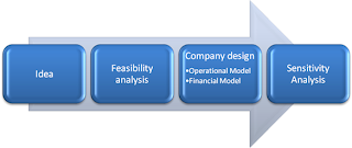
Operational Models

1.       Staffing model

2.       Revenue model

3.       Cost of goods sold model

4.       Cost of sales and marketing model

5.       Cost of product development model

6.       Cost of operating expenses model

7.       Capital expenditure model

 

Financial Model

1.       Statement of profit and loss

2.       Statement of cash flows

3.       Investment and valuation model

4.       Balance Sheet

 

Operational Project Planning

 

1.       Define the purpose of the project (company):

 

 

2.       Define the Scope:

 

 

3.       Define the names

 

 

4.       Define assumptions and risks

 

 

5.       Define roles and responsibilities

 

 

6.       Define the master schedule and milestones

 

 

On the basis of the above business planning; we have to plan the financials with the business potential and demand analysis data.

 

Will continue,……………..

Nested IF statements in a Cell of a worksheet

One of my friend asked me; how many IF statements can I nest in a cell?

 

Interesting, It is 64 IF statements in  a cell (version 2007 and above)

 

In excel version 2007, a cell can contain up to 32,000 characters.