Customizing the chart to prepare a professional presentation

Question: How do I customize the chart for the meaningful presentation

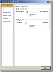
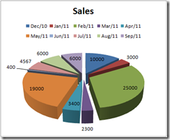
Answer: In Excel 2007 and above the charts can be easily customized with the command Format object (chart).  This is a common window have the properties needs to be changed.  In the below example the pie chart pan and pan explosion angle can be rotated by the properties window.

Copy paste the data in a excel sheet and select the data to insert the pie chart.

Sl No.	Month	Sales
1	Dec/10	10000
2	Jan/11	3000
3	Feb/11	25000
4	Mar/11	2300
5	Apr/11	3400
6	May/11	19000
7	Jun/11	400
8	Jul/11	4567
9	Aug/11	6000
10	Sep/11	6000

 

Right click the chart and select the format command.  In the menu select your choice and customize the chart as required and give a professional look.

How to Add the visible rows values in a list - MS Excel 2003, 2007, 2010

Questions :  Teacher want to put the total of the marks in a list of all students in the school.  He want to use the filter to get the data of class; section and subjects.

Solutions :  Use the '=SUBTOTAL(9,E8:E61)' to get the desired result.

Step 1:  Open the list of values
Step 2:  Select all the data and apply the auto filter function.  Short cut Alt D, F, F.
Step 3:  Goto the last cell of the column where the marks ends.
Step 4:  In the next row use the Auto sum function. Short cut 'Alt =' and press enter key.
Step 5:  Excel will build the subtotal function since the filter is applied in the data.
Step 6:  Change the reference series in the function as required to calculate the sum of marks in the visible cells.

Copy and paste the formula in a excel sheet tips - Relative and Absolute references

Question : How do we enter a formula in a sheet can be copy - pasted to other cells.  I am not getting the desired result in one shot and I need to change the formula after the paste activity.  Need a short cut to do it in one shot;

Answer : In excel we can use to types of reference i.e. absolute reference and relative reference.

Absolute Reference - will not change the focus while doing the copy and paste activity.  To do this use the '$' symbol in the formula.  The shortcut key is 'F4' key in the keyboard.  Press number of time to Toggle from freeze and non freeze the reference.

Relative Reference - This is the default option and when you copy and paste excel will automatically changes the references with respect to the movement of destination cell.

Example :

	E	F	G	H
	Amount	Running Sum	Discount	0.1
5	1446.94	=E5	=E5*$H$4
6	2135.89	=E6+F5	=E6*$H$4
7	1258.26	=E7+F6	=E7*$H$4
8	2137.48	=E8+F7	=E8*$H$4
9	2137.48	=E9+F8	=E9*$H$4
10	2137.48	=E10+F9	=E10*$H$4
11	2137.47	=E11+F10
12	1259.19	=E12+F11
13	1259.19	=E13+F12
14	1259.19	=E14+F13
15	1259.19	=E15+F14
16	1573.99	=E16+F15

 
The formula in the F column is in relative reference formula.
The formula in the G column is in absolute reference formula.

How to find the duplicate records in the database

My friends question;  Which is the method, good to find the duplicate records in the set of records entered in a worksheet.

Answer:

There are various methods followed to find the duplicate records in a database stored in a excel.

a.  In Excel 2007 and above, Conditional Formatting  is the easiest way.

b.  Use the 'countif' formula

c.  Use  a Pivot table function

d.  Use  Subtotal function

e.  Use Advanced filter

f.    Remove duplicate button  Alt A, M 

User has to chose the appropriate method to find the duplicate records. 

How to find the Principle and Interest component in monthly equal monthly installment by MS Excel 2010

Questions :  My friend has a request to create a sheet in which he wants to find the interest and principle component in his equal monthly installment on all the payment schedule.

My Solution :
Excel has a build in function PPMT() to find principle part of the EMI paid by him.  The PMT() Function will be used for find the EMI Value of the loan part.

The steps to create the sheet is;

A	B	C	D	E	F	G	H
5
6	Loan Amount	(5,00,000)
7	Term	18	Months
8	Rate	14%
9
10	PMT	Rs.30,958	=PMT(C8/12,C7,C6,0)
11				=PPMT($C$8/12,$C13,$C$7,$C$6)
12		Payment	Date	Principal	Interest	Balance
13		1	1-Dec-10	25,124	5,833	25,124
14		2	1-Jan-11	25,417	5,540	50,542
15		3	1-Feb-11	25,714	5,244	76,256
16		4	1-Mar-11	26,014	4,944	1,02,269
17		5	1-Apr-11	26,317	4,640	1,28,587
18		6	1-May-11	26,624	4,333	1,55,211
19		7	1-Jun-11	26,935	4,023	1,82,146
20		8	1-Jul-11	27,249	3,708	2,09,396
21		9	1-Aug-11	27,567	3,390	2,36,963
22		10	1-Sep-11	27,889	3,069	2,64,852
23		11	1-Oct-11	28,214	2,743	2,93,066
24		12	1-Nov-11	28,543	2,414	3,21,609
25		13	1-Dec-11	28,876	2,081	3,50,486
26		14	1-Jan-12	29,213	1,744	3,79,699
27		15	1-Feb-12	29,554	1,404	4,09,253
28		16	1-Mar-12	29,899	1,059	4,39,152
29		17	1-Apr-12	30,248	710	4,69,399
30		18	1-May-12	30,601	357	5,00,000

Step 1:  Enter the Loan amount in negative in a cell
Step 2 : Enter the Payment terms and rate of interest to be paid
Step 3: Use the PMT function to find the equal monthly installment "

=PMT(C8/12,C7,C6,0)"

Step 4: Create a table to find the every month principle with function. "=PPMT($C$8/12,$C13,$C$7,$C$6)"
 Step 5:  The interest component can be calculated by the formula "=$C$10-E13"
Step 6 :  The remaining outstanding value of the loan value will be estimated by the formula =$C$2+E13
Step 7 : Copy and paste the value above in a sheet and paste it in a excel sheet to understand the functions.

Please post your comments to make it useful for our friends. 

How to find absent date

My HR friend Question:

He got the personnel data from Time office in a excel book.  The book has number of sheets belongs to various employee attendance, i.e. one sheet for each employee.  The data has date and time recorded by the system on use of punch card / Tag.

My Solution:

He can use the 'Networkdays' function to find the missing dates. Please follow the below steps

Step1 : Insert a column next to present dates
Step 2 : Use the function - "=NETWORKDAYS(H5,H6,"Holidayrange")"
Step 3 : Copy and paste the function for all rows
Step 4 :  If value is 2 then he is continuously present. If value is more than 2 the he has taken leave in the period. 

Note - The function is applicable for five day working only. It will calculate Monday to Friday has working days.

Define holiday in Named range and use it any where in the workbook

My HR Friend:

HR prepares the time office report for all the employees in a excel sheet.  He is using the Networking days function to find the working days in the month and calculates the salary for the month.  He is manually entering the holidays in the formula and finding difficult that the holidays not accounted because of format error while typing it in the function.

My Solution is:

One can create a named range in the beginning of year and save the holidays a 'Named Range' and call it to the Networkdays function. The steps for creating the named ranged is given below;

STEPS
Step 1:	Type your name holidays as a column of dates in A6:A13
Step 2:	In a blank cell,type=A6:A13.Do not press enter instead,press the F9 key.
	{40923;40934;41013;41030;41136;41164;41192;41226}
Step 3:	Press ctrl+C to copy the array to the clipboard.
Step 4:	Press Esc to exit formula Edit mode.The formula disappears
Step 5:	Visit the name dialog box (Formula->Define name)
Step 6:	Type Holidays as the name.
Step 7:	In the refes to Box,clear the current text.Type an equals sign.Press Ctrl+V to paste the array of dates to the box.Click ok.

Trend graph for analysis

Question :
I have used a trend graph for the plan and actual sale values.  I am not getting the graph as required. How to do it?

Solution:

For trend graph we need to use the cumulative value rather than monthly value to get the desired graphs.

The cumulative values will represents the progressive value to achieve at different point of time.

	Plan	Cplan	Actual	Cactual
Jan	10	10	10	10
Feb	12	22	13	23
Mar	12	34	14	37
Apr	12	46	11	48
May	18	64	23	71
Jun	20	84	30	101
Jul	20	104	20	121
Aug	20	124	19	140
Sep	20	144	15	155
Oct	20	164	18	173
Nov	20	184	22	195
Dec	20	204	30	225

How do I find duplicate payment vouchers made for a invoice

My friend problem is :

My friend Team Leader has to supervise the indexing work for the invoices received and create payment vouchers in the ERP by his team members.  He can drill down the indexed vouchers for the day / week.  Every voucher has multiple line items indexed on the basis of a invoice.

My Solutions is;

Step 1 : Drill down the dump from your ERP

Step 2 : Use the Pivot table and sum the value of amount on the basis of invoice and voucher.

Step 3 : It will clearly show the duplicate vouchers if any indexed.  See the picture.

Also we can use the Report filter function in the Pivot table to filter the invoice in the dump and clear the duplicate payment.

How do I find a date after 3 months from today?

Question;

My friend had a situation that he want create a sheet that every forth month on the same date of billing the customer needs to be remained for their premium payment.  He want a function to use in his formula since their are 300 customer he need to send advice on next billing.

My Solution is;

Step 1 : Customer are need to be reminded for their premium payment on quarterly basis.  In a column put the billing date.

Step 2 : Create a column to find the date on which the reminder has to be send.

Step 3 : If  D1 has the billing date; the function/formula at E1 is;
=DATE(YEAR(D1),MONTH(D1)+3,DAY(D1))

Step 4:  Copy the formula for all the rows which will give you the next billing date. 

How do excel update the summary sheet in a visit plan

Question;
One of my friend has a question; He had prepared a list of companies in a excel sheet to prepare a visit plan.
Now he had made a color coding Blue; Red and Green to represent Plan, not visited and visited respectively.  He want to prepare a report summary for the visit report.

My Solution is ;
Step 1:  Use find and replace commend - to find the color format and replace all with 'B' for blue color; 'R' for Red and G for Green.

Step 2:  Insert a summary sheet and use the color code and design as you need to present to you management

Step 3:  Use count if formula to count the value of 'B', 'R' and 'G'.

Step 4:  He continue the plan visual chart as it is and the summary will change dynamically as he updates the report.

How is it!!!!